There is some empirical evidence that Bayesian networks are not too sensitive to parameters; this is due to the fact that many classic examples of Bayesian networks are sparse graphs, with probability values that are close to zero or one (for example, noisy functions have probability values that are only zero or one). When that happens, you're lucky because robustness is likely to be present. In other words, if changes in one variable do not affect many variables, and changes are not large relative to the magnitude of the numbers, then it is likely that these changes will not produce significant variations in inferences.
Situations where probability values are not very close to zero-one, or where the graph is heavily inter-connected, are situations where robustness may falter. Another situation is model building, where some parameter are not entirely specified, and the question is how much effort should be spent nailing down their values. A serious analysis of a network must consider the possibility of robustness problems, or at least assess how robust the model is. That's the aspect of inference that JavaBayes is trying to address.
Research on Bayesian networks has not fully explored the robustness analysis aspect of inference, due to the lack of algorithms for inferences with convex sets of distributions. JavaBayes is the first Bayesian network engine that provides facilities that explicitly account for perturbations in probabilistic models.
JavaBayes contains two classes of algorithms for robustness analysis:
The algorithms in JavaBayes employ some recent results to reduce the complexity of robustness analysis. The starting point is the theory of Quasi-Bayesian behavior, proposed in 1980 by Giron and Rios. This theory builds a complete decision making model based on convex sets of probability measures.
A complete discussion of all these issues and an exposition of algorithms can be found at http://www.cs.cmu.edu/~qbayes/Tutorial/.
Suppose you set a network to represent a multivariate constant density ratio class. You can do this in the Edit Network dialog. If you save the network with the global neighborhood set (in the BIF 0.15 format), you should see the property:
network Example {
	property credal-set constant-density-ratio 1.2;
}
When an inference is requested, the algorithm for global neighborhoods
with density ratio classes will be called. The parameter that defines
the class in the example is 1.2. If this parameter is smaller
than zero, the parameter is automatically set to one (so that it
has no effect); if it is smaller than one, then its inverse
is used (the parameter has to be larger than one).
Take another example. Suppose a network is declared with the credal-set epsilon-contaminated property:
network Example {
	property credal-set epsilon-contaminated 0.1;
}
then the algorithm for global neighborhoods with
epsilon-contaminated
classes will be called, using 0.1 as the definition parameter for the
epsilon-contaminated class. If this parameter is smaller than zero or
larger than one, inferences assume the parameter to be zero.
There are four possible global neighborhoods for a network:
network Example {
	property credal-set constant-density-ratio 1.1;
}

network Example {
	property credal-set epsilon-contaminated 0.1;
}

network Example {
	property credal-set constant-density-bounded 1.1;
}

network Example {
	property credal-set total-variation 0.1;
}
The parameter for the constant density bounded class behaves as
the parameter for the constant density ratio class;
the parameter for the total variation class behaves as
the parameter for the
epsilon-contaminated class.
If any of the credal-set properties above are present, the result is a pair of functions, the lower and the upper bounds for the posterior marginals.
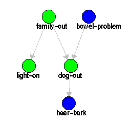
Consider the example discussed in Section 5.1, taken from [4].
|
Posterior distribution:
probability (  "light-on" ) { //1 variable(s) and 2 values
	table 0.23651916875671802 0.763480831243282 ;
}
Now try to perform a robustness analysis by adding say an
epsilon-contamination of 0.1. This roughly means that you expect the
Bayesian network description to be correct 90 percent of the time, but
in 10 percent of the cases you would expect any other joint distribution
to be possible. Notice this is a somewhat radical model of uncertainty
as you are allowing for 0.1 in probability mass to be concentrated in
arbitrary sets or events. Add the following line in the network block:
property credal-set epsilon-contaminated 0.1;and load the new network description into JavaBayes: You will get the result:
Posterior distribution:
 envelope (  "light-on" ) { //1 variable(s) and 2 values
	table lower-envelope 0.21286725188104622 0.6871327481189539 ;
	table upper-envelope 0.31286725188104625 0.7871327481189538 ;
}
These functions are the lower and upper bounds respectively.
To associate a variable with a set of densities, you have to insert the vertices of the set of densities. Go to the Edit variable window and mark some variable as a Credal set with extreme points. Insert the number of vertices of the set of distributions. Then edit these densities in the Edit function window.
You can also insert the vertices of a set of densities directly into the describing a network; JavaBayes simply asks you to determine which vertice you are referring to. In the example above, suppose you want to define an interval for the probability of family-out. You can write a file in the BIF0.15 format with the following declaration:
probability ( "family-out" ) { //1 variable(s) and 2 values
	table 0.15 0.85 ;
	table 0.25 0.75 ;
}
This defines an interval
If you insert the set of densities above, then you get:
Posterior distribution:
 envelope (  "light-on"  "<Transparent:family-out>" ) { //2 variable(s) and 2 values
	table lower-envelope 0.23651916875671802 0.6792901716068643 ;
	table upper-envelope 0.3207098283931358 0.763480831243282 ;
}
This indicates the lower and upper bounds for the probability
of light-on given the evidence, and also indicates which sets
of densities affect the result (in this case, the
densities for family-out).